季節調整済みARIMAモデルで電力使用状況を推定してみる
北海道電力の電力使用状況を季節調整済みARIMAモデル(Seasonal ARIMA)で推定してみました。そのメモです。
このサイトを参考にしました。ほぼそのままやりました。
■Seasonal ARIMA with Python
http://www.seanabu.com/2016/03/22/time-series-seasonal-ARIMA-model-in-python/
このブログでも紹介されていますが、statsmodelsのdevelopment versionが必要です。
https://github.com/statsmodels/statsmodels
これをインストールするにはvisual c++のなんかのバージョンが必要で色々と面倒でした。あと、pipでインストールすると失敗するのでeasy_installでうまくいく場合もありました。
%pylab
import pandas as pd
import numpy as np
import matplotlib.pyplot as plt
import datetime
from dateutil.relativedelta import relativedelta
import seaborn as sns #グラフが見やすくなる
import statsmodels.api as sm
from statsmodels.tsa.stattools import acf
from statsmodels.tsa.stattools import pacf
from statsmodels.tsa.seasonal import seasonal_decompose
data = pd.read_csv("http://denkiyoho.hepco.co.jp/data/2016_juyo_hokkaidou.csv", skiprows=3,names=['Date','Time','power'])
data.index = pd.to_datetime(data['Date'])
df = data.groupby(data.index).mean()
df['power'] = df.power.apply(lambda x: int(x)*10000)
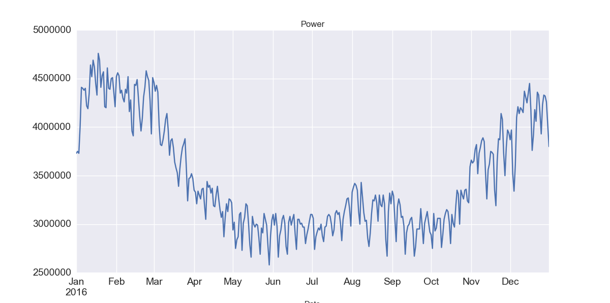
df.power.plot(figsize=(12,6), title= 'Power', fontsize=14)
まず取得したデータをグラフにしてみました。
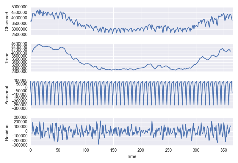
ここからトレンド、季節変動、、残差(ランダム成分)にわけます。
plt.close()

df = pd.DataFrame(df['power'].values.astype(int), pd.DatetimeIndex(start='2016-01-01', periods=len(df['power']), freq='D'))
df.columns= ['power']
decomposition = seasonal_decompose(df.values, freq=7)
fig = plt.figure()
fig = decomposition.plot()
fig.set_size_inches(8, 8)
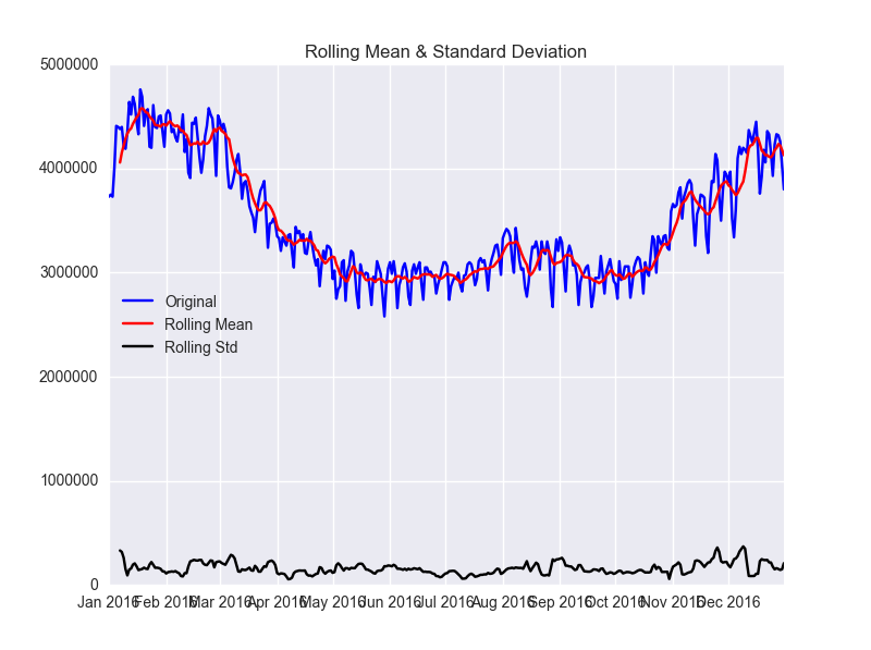
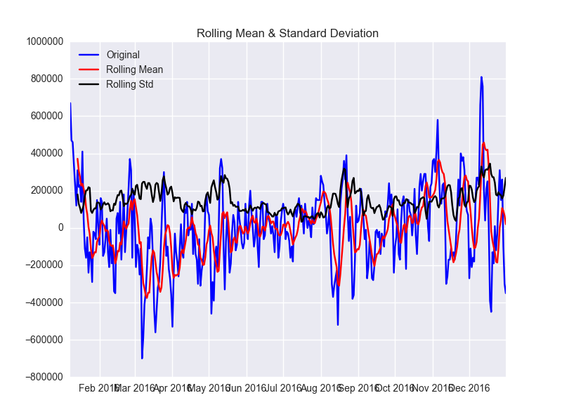
ここから定常性を確認します。参考にした記事に良いものがありましたので使わせてもらいます。
plt.close()

from statsmodels.tsa.stattools import adfuller
def test_stationarity(timeseries):

    #Determing rolling statistics
    rolmean = pd.rolling_mean(timeseries, window=7)
    rolstd = pd.rolling_std(timeseries, window=7)

    #Plot rolling statistics:
    fig = plt.figure(figsize=(8, 6))
    orig = plt.plot(timeseries, color='blue',label='Original')
    mean = plt.plot(rolmean, color='red', label='Rolling Mean')
    std = plt.plot(rolstd, color='black', label = 'Rolling Std')
    plt.legend(loc='best')
    plt.title('Rolling Mean & Standard Deviation')
    plt.show()

    #Perform Dickey-Fuller test:
    print ("Results of Dickey-Fuller Test:")
    dftest = adfuller(timeseries, autolag='AIC')
    dfoutput = pd.Series(dftest[0:4], index=['Test Statistic','p-value','#Lags Used','Number of Observations Used'])
    for key,value in dftest[4].items():
        dfoutput['Critical Value (%s)'%key] = value
    print (dfoutput)

test_stationarity(df.power)

###Results of Dickey-Fuller Test:###
Test Statistic                  -1.832150
p-value                          0.364621
#Lags Used                      14.000000
Number of Observations Used    351.000000
Critical Value (1%)             -3.449119
Critical Value (5%)             -2.869810
Critical Value (10%)            -2.571176
dtype: float64
データは定常性ではないことがわかります。
次に1次の差分をとった場合です。
plt.close()

df['first_difference'] = df.power - df.power.shift(1)
test_stationarity(df.first_difference.dropna(inplace=False))

###Results of Dickey-Fuller Test:###
Test Statistic                -5.660888e+00
p-value                        9.385886e-07
#Lags Used                     1.300000e+01
Number of Observations Used    3.510000e+02
Critical Value (1%)           -3.449119e+00
Critical Value (5%)           -2.869810e+00
Critical Value (10%)          -2.571176e+00
dtype: float64
まだまだ定常性ではないです。
次は季節性の差分をとります。
plt.close()

df['seasonal_difference'] = df.power - df.power.shift(7)
test_stationarity(df.seasonal_difference.dropna(inplace=False))

###Results of Dickey-Fuller Test:###
Test Statistic                  -3.452940
p-value                          0.009281
#Lags Used                      14.000000
Number of Observations Used    344.000000
Critical Value (1%)             -3.449503
Critical Value (5%)             -2.869979
Critical Value (10%)            -2.571266
dtype: float64
よくなりましたがまだまだです。
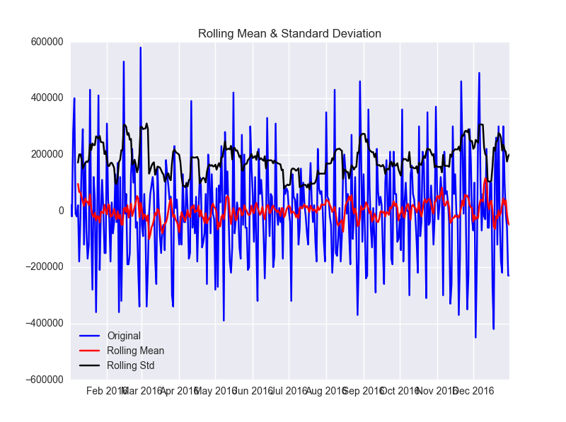
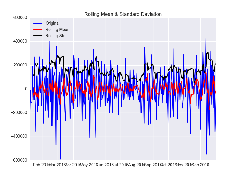
一次の差分と、季節性を取り除きます。
plt.close()

df['seasonal_first_difference'] = df.first_difference - df.first_difference.shift(7)
test_stationarity(df.seasonal_first_difference.dropna(inplace=False))

###Results of Dickey-Fuller Test:###
Test Statistic                -9.147004e+00
p-value                        2.750689e-15
#Lags Used                     1.300000e+01
Number of Observations Used    3.440000e+02
Critical Value (1%)           -3.449503e+00
Critical Value (5%)           -2.869979e+00
Critical Value (10%)          -2.571266e+00
dtype: float64
これでまあよくなりました。
ACFとPACFからパラメータを選びます。
plt.close()

fig = plt.figure(figsize=(8,6))
ax1 = fig.add_subplot(211)
fig = sm.graphics.tsa.plot_acf(df.seasonal_first_difference.iloc[8:], lags=40, ax=ax1)
ax2 = fig.add_subplot(212)
fig = sm.graphics.tsa.plot_pacf(df.seasonal_first_difference.iloc[8:], lags=40, ax=ax2)
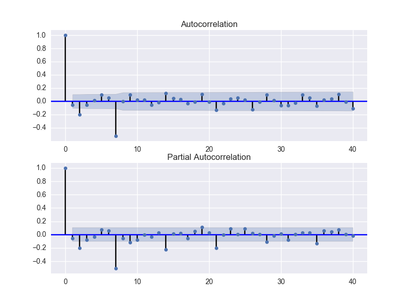
こちらを参考にモデルのパラメータを選べばいいそうです。
■ARIMA models for time series forecasting
http://people.duke.edu/~rnau/arimrule.htm
もっと簡単にパラメータを選ぶ方法があればいいと思いますが、ないんですかね?
seasonal_order=(0,1,1,7)とseasonal_order=(1,1,1,7)でモデルを作成してみました。
plt.close()

mod = sm.tsa.statespace.SARIMAX(df.power, trend='n', order=(0,1,0), seasonal_order=(0,1,1,7))
results = mod.fit()
print (results.summary())


                                 Statespace Model Results
=========================================================================================
Dep. Variable:                             power   No. Observations:                  366
Model:             SARIMAX(0, 1, 0)x(0, 1, 1, 7)   Log Likelihood               -4772.423
Date:                           Thu, 09 Mar 2017   AIC                           9548.846
Time:                                   21:04:58   BIC                           9556.607
Sample:                               01-01-2016   HQIC                          9551.932
                                    - 12-31-2016
Covariance Type:                             opg
==============================================================================
                 coef    std err          z      P>|z|      [0.025      0.975]
------------------------------------------------------------------------------
ma.S.L7       -0.4498      0.012    -36.021      0.000      -0.474      -0.425
sigma2      1.674e+10    2.7e-13   6.21e+22      0.000    1.67e+10    1.67e+10
===================================================================================
Ljung-Box (Q):                       50.61   Jarque-Bera (JB):              1021.36
Prob(Q):                              0.12   Prob(JB):                         0.00
Heteroskedasticity (H):               0.52   Skew:                            -1.32
Prob(H) (two-sided):                  0.00   Kurtosis:                        10.84
===================================================================================

Warnings:
[1] Covariance matrix calculated using the outer product of gradients (complex-step).
[2] Covariance matrix is singular or near-singular, with condition number 1.36e+37. Standard errors may be unstable.
mod = sm.tsa.statespace.SARIMAX(df.power, trend='n', order=(0,1,0), seasonal_order=(1,1,1,7))
results = mod.fit()
print (results.summary())


                                 Statespace Model Results
=========================================================================================
Dep. Variable:                             power   No. Observations:                  366
Model:             SARIMAX(0, 1, 0)x(1, 1, 1, 7)   Log Likelihood               -4745.075
Date:                           Thu, 09 Mar 2017   AIC                           9496.150
Time:                                   21:06:44   BIC                           9507.792
Sample:                               01-01-2016   HQIC                          9500.780
                                    - 12-31-2016
Covariance Type:                             opg
==============================================================================
                 coef    std err          z      P>|z|      [0.025      0.975]
------------------------------------------------------------------------------
ar.S.L7        0.4606      0.020     22.704      0.000       0.421       0.500
ma.S.L7       -0.9589      0.030    -32.239      0.000      -1.017      -0.901
sigma2      1.614e+10   2.89e-13   5.57e+22      0.000    1.61e+10    1.61e+10
===================================================================================
Ljung-Box (Q):                       88.63   Jarque-Bera (JB):                 7.99
Prob(Q):                              0.00   Prob(JB):                         0.02
Heteroskedasticity (H):               0.63   Skew:                            -0.26
Prob(H) (two-sided):                  0.01   Kurtosis:                         3.52
===================================================================================

Warnings:
[1] Covariance matrix calculated using the outer product of gradients (complex-step).
[2] Covariance matrix is singular or near-singular, with condition number    inf. Standard errors may be unstable.
seasonal_order=(1,1,1,7)のほうがAICとBICの値が小さくなっていましたのでseasonal_order=(1,1,1,7)でグラフにしてみます。
fig, ax = plt.subplots()
ax.set(title='HOKKAIDO POWER', xlabel='Date', ylabel='Power')
ax.plot(df.power.ix['2016-01-01':], 'g',label="power",color="darkgrey")
ax.plot(results.predict(start = 364, end= 380, dynamic= True),'g',label="forcast",color="green")
legend = ax.legend(loc='lower right')
legend.get_frame().set_facecolor('w')
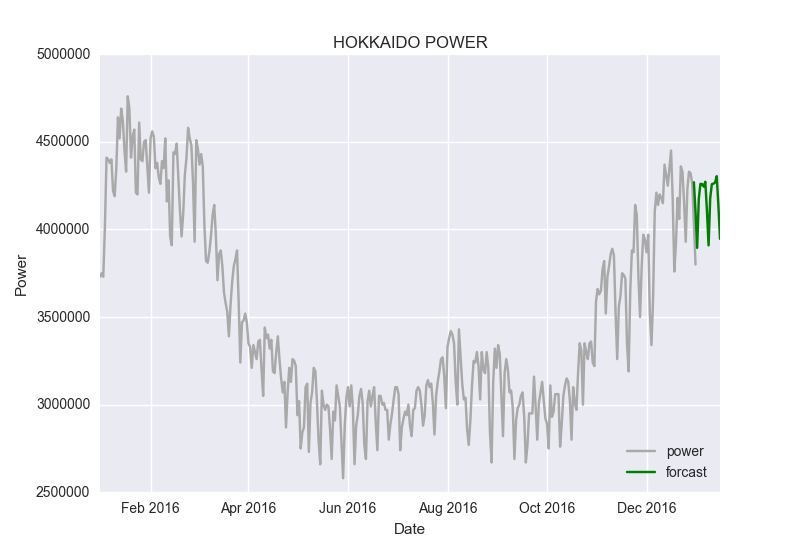
ほほーという感じですね。もう少しいろいろなデータで検証してみたいと思います。
※参考
■Statsmodels Examples
http://www.statsmodels.org/devel/examples/index.html
■Rで季節変動のある時系列データを扱ってみる
http://tjo.hatenablog.com/entry/2013/10/30/190552
関連する投稿:
- 2017-02-11:Python3でビットコインの回帰線を描いてみる
- 2017-03-14:季節調整済みARIMAモデルで電力使用状況を推定してみる part2 予測表示
- 2017-01-25:軍需企業の株価
- 2017-03-17:SARIMAXモデルでPVを予測してみる
- 2017-02-24:電力データから季節変動の分解
“季節調整済みARIMAモデルで電力使用状況を推定してみる” への2件の返信